This example has been auto-generated from the examples/ folder at GitHub repository.
Autoregressive Models
# Activate local environment, see `Project.toml`
import Pkg; Pkg.activate(".."); Pkg.instantiate();
In this example we are going to perform an automated Variational Bayesian Inference for a latent autoregressive model that can be represented as following:
\[\begin{aligned} p(\gamma) &= \mathrm{Gamma}(\gamma|a, b),\\ p(\mathbf{\theta}) &= \mathcal{N}(\mathbf{\theta}|\mathbf{\mu}, \Sigma),\\ p(x_t|\mathbf{x}_{t-1:t-k}) &= \mathcal{N}(x_t|\mathbf{\theta}^{T}\mathbf{x}_{t-1:t-k}, \gamma^{-1}),\\ p(y_t|x_t) &= \mathcal{N}(y_t|x_t, \tau^{-1}), \end{aligned}\]
where $x_t$ is a current state of our system, $\mathbf{x}_{t-1:t-k}$ is a sequence of $k$ previous states, $k$ is an order of autoregression process, $\mathbf{\theta}$ is a vector of transition coefficients, $\gamma$ is a precision of state transition process, $y_k$ is a noisy observation of $x_k$ with precision $\tau$.
For a more rigorous introduction to Bayesian inference in Autoregressive models we refer to Albert Podusenko, Message Passing-Based Inference for Time-Varying Autoregressive Models.
We start with importing all needed packages:
using RxInfer, Distributions, LinearAlgebra, Random, Plots, BenchmarkTools, ParametersLet's generate some synthetic dataset, we use a predefined sets of coeffcients for $k$ = 1, 3 and 5 respectively:
# The following coefficients correspond to stable poles
coefs_ar_1 = [-0.27002517200218096]
coefs_ar_2 = [0.4511170798064709, -0.05740081602446657]
coefs_ar_5 = [0.10699399235785655, -0.5237303489793305, 0.3068897071844715, -0.17232255282458891, 0.13323964347539288];
function generate_ar_data(rng, n, θ, γ, τ)
order = length(θ)
states = Vector{Vector{Float64}}(undef, n + 3order)
observations = Vector{Float64}(undef, n + 3order)
γ_std = sqrt(inv(γ))
τ_std = sqrt(inv(τ))
states[1] = randn(rng, order)
for i in 2:(n + 3order)
states[i] = vcat(rand(rng, Normal(dot(θ, states[i - 1]), γ_std)), states[i-1][1:end-1])
observations[i] = rand(rng, Normal(states[i][1], τ_std))
end
return states[1+3order:end], observations[1+3order:end]
endgenerate_ar_data (generic function with 1 method)# Seed for reproducibility
seed = 123
rng = MersenneTwister(seed)
# Number of observations in synthetic dataset
n = 500
# AR process parameters
real_γ = 1.0
real_τ = 0.5
real_θ = coefs_ar_5
states, observations = generate_ar_data(rng, n, real_θ, real_γ, real_τ);Let's plot our synthetic dataset:
plot(first.(states), label = "Hidden states")
scatter!(observations, label = "Observations")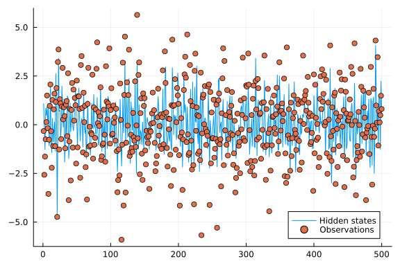
Next step is to specify probabilistic model, inference constraints and run inference procedure with RxInfer. We will specify two different models for Multivariate AR with order $k$ > 1 and for Univariate AR (reduces to simple State-Space-Model) with order $k$ = 1.
@model function lar_model(T, y, order, c, τ)


    # Prior for first state
    if T === Multivariate
        γ  ~ Gamma(α = 1.0, β = 1.0)
        θ  ~ MvNormal(μ = zeros(order), Λ = diageye(order))
        x0 ~ MvNormal(μ = zeros(order), Λ = diageye(order))
    else
        γ  ~ Gamma(α = 1.0, β = 1.0)
        θ  ~ Normal(μ = 0.0, γ = 1.0)
        x0 ~ Normal(μ = 0.0, γ = 1.0)
    end

    x_prev = x0

    for i in eachindex(y)

        x[i] ~ AR(x_prev, θ, γ)

        if T === Multivariate
            y[i] ~ Normal(μ = dot(c, x[i]), γ = τ)
        else
            y[i] ~ Normal(μ = c * x[i], γ = τ)
        end

        x_prev = x[i]
    end

end
@constraints function ar_constraints()
q(x0, x, θ, γ) = q(x0, x)q(θ)q(γ)
endar_constraints (generic function with 1 method)@meta function ar_meta(artype, order, stype)
AR() -> ARMeta(artype, order, stype)
endar_meta (generic function with 1 method)@initialization function ar_init(morder)
q(γ) = GammaShapeRate(1.0, 1.0)
q(θ) = MvNormalMeanPrecision(zeros(morder), diageye(morder))
endar_init (generic function with 1 method)morder = 5
martype = Multivariate
mc = ReactiveMP.ar_unit(martype, morder)
mconstraints = ar_constraints()
mmeta = ar_meta(martype, morder, ARsafe())
moptions = (limit_stack_depth = 100, )
mmodel = lar_model(T=martype, order=morder, c=mc, τ=real_τ)
mdata = (y = observations, )
minitialization = ar_init(morder)
mreturnvars = (x = KeepLast(), γ = KeepEach(), θ = KeepEach())
# First execution is slow due to Julia's initial compilation
# Subsequent runs will be faster (benchmarks are below)
mresult = infer(
model = mmodel,
data = mdata,
constraints = mconstraints,
meta = mmeta,
options = moptions,
initialization = minitialization,
returnvars = mreturnvars,
free_energy = true,
iterations = 50,
showprogress = false
);@unpack x, γ, θ = mresult.posteriorsDict{Symbol, Vector} with 3 entries:
:γ => GammaShapeRate{Float64}[GammaShapeRate{Float64}(a=251.0, b=47.5918)
, Ga…
:θ => MvNormalWeightedMeanPrecision{Float64, Vector{Float64}, Matrix{Floa
t64}…
:x => MvNormalWeightedMeanPrecision{Float64, Vector{Float64}, Matrix{Floa
t64}…We will use different initial marginals depending on type of our AR process
p1 = plot(first.(states), label="Hidden state")
p1 = scatter!(p1, observations, label="Observations")
p1 = plot!(p1, first.(mean.(x)), ribbon = first.(std.(x)), label="Inferred states", legend = :bottomright)

p2 = plot(mean.(γ), ribbon = std.(γ), label = "Inferred transition precision", legend = :topright)
p2 = plot!([ real_γ ], seriestype = :hline, label = "Real transition precision")

p3 = plot(mresult.free_energy, label = "Bethe Free Energy")

plot(p1, p2, p3, layout = @layout([ a; b c ]))
Let's also plot a subrange of our results:
subrange = div(n,5):(div(n, 5) + div(n, 5))

plot(subrange, first.(states)[subrange], label="Hidden state")
scatter!(subrange, observations[subrange], label="Observations")
plot!(subrange, first.(mean.(x))[subrange], ribbon = sqrt.(first.(var.(x)))[subrange], label="Inferred states", legend = :bottomright)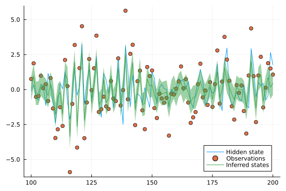
It is also interesting to see where our AR coefficients converge to:
let
    pθ = plot()

    θms = mean.(θ)
    θvs = var.(θ)

    l = length(θms)

    edim(e) = (a) -> map(r -> r[e], a)

    for i in 1:length(first(θms))
        pθ = plot!(pθ, θms |> edim(i), ribbon = θvs |> edim(i) .|> sqrt, label = "Estimated θ[$i]")
    end

    for i in 1:length(real_θ)
        pθ = plot!(pθ, [ real_θ[i] ], seriestype = :hline, label = "Real θ[$i]")
    end

    plot(pθ, legend = :outertopright, size = (800, 300))
end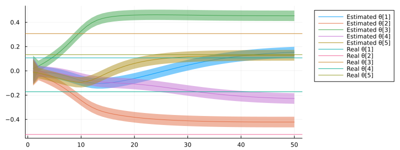
println("$(length(real_θ))-order AR inference Bethe Free Energy: ", last(mresult.free_energy))5-order AR inference Bethe Free Energy: 1024.077566129808We can also run a 1-order AR inference on 5-order AR data:
uorder  = 1
uartype = Univariate
uc      = ReactiveMP.ar_unit(uartype, uorder)
uconstraints = ar_constraints()
umeta        = ar_meta(uartype, uorder, ARsafe())

uoptions = (limit_stack_depth = 100, )
umodel         = lar_model(T=uartype, order=uorder, c=uc, τ=real_τ)
udata          = (y = observations, )
initialization = @initialization begin
    q(γ) = GammaShapeRate(1.0, 1.0)
    q(θ) = NormalMeanPrecision(0.0, 1.0)
end
ureturnvars    = (x = KeepLast(), γ = KeepEach(), θ = KeepEach())

uresult = infer(
    model = umodel,
    data  = udata,
    meta  = umeta,
    constraints    = uconstraints,
    initialization = initialization,
    returnvars     = ureturnvars,
    free_energy    = true,
    iterations     = 50,
    showprogress   = false
);
println("1-order AR inference Bethe Free Energy: ", last(uresult.free_energy))1-order AR inference Bethe Free Energy: 1025.8792949319945if uresult.free_energy[end] > mresult.free_energy[end]
println("We can see that, according to final Bethe Free Energy value, in this example 5-order AR process can describe data better than 1-order AR.")
else
error("AR-1 performs better than AR-5...")
endWe can see that, according to final Bethe Free Energy value, in this exampl
e 5-order AR process can describe data better than 1-order AR.Autoregressive Moving Average Model
Bayesian ARMA model can be effectively implemeted in RxInfer.jl. For theoretical details on Varitional Inference for ARMA model, we refer the reader to the following paper. The Bayesian ARMA model can be written as follows:
\[\begin{aligned} e_t \sim \mathcal{N}(0, \gamma^{-1}) \quad \theta &\sim \mathcal{MN}(\mathbf{0}, \mathbf{I}) \quad \eta \sim \mathcal{MN}(\mathbf{0}, \mathbf{I}) \\ \mathbf{h}_0 &\sim \mathcal{MN}\left(\begin{bmatrix} e_{-1} \\ e_{-2} \end{bmatrix}, \mathbf{I}\right) \\ \mathbf{h}_t &= \mathbf{S}\mathbf{h}_{t-1} + \mathbf{c} e_{t-1} \\ \mathbf{x}_t &= \boldsymbol{\theta}^\top\mathbf{x}_{t-1} + \boldsymbol{\eta}^\top\mathbf{h}_{t} + e_t \end{aligned}\]
where shift matrix $\mathbf{S}$ is
\[\begin{aligned} \mathbf{S} = \begin{pmatrix} 0 & 0 \\ 1 & 0 \end{pmatrix} \end{aligned}\]
and unit vector $\mathbf{c}$:
\[\begin{aligned} \mathbf{c}=[1, 0] \end{aligned}\]
when MA order is $2$
In this way, $\mathbf{h}_t$ containing errors $e_t$ can be viewed as hidden state.
In short, the Bayesian ARMA model has two intractabilities: (1) induced by the multiplication of two Gaussian RVs, i.e., $\boldsymbol{\eta}^\top\mathbf{h}_{t}$, (2) induced by errors $e_t$ that prevents analytical update of precision parameter $\gamma$ (this can be easily seen when constructing the Factor Graph, i.e. there is a loop). Both problems can be easily resolved in RxInfer.jl, by creating a hybrid inference algorithm based on Loopy Variational Message Passing.
# Load packages
using RxInfer, LinearAlgebra, CSV, DataFrames, Plots
# Define shift function
function shift(dim)
S = Matrix{Float64}(I, dim, dim)
for i in dim:-1:2
S[i,:] = S[i-1, :]
end
S[1, :] = zeros(dim)
return S
endshift (generic function with 1 method)@model function ARMA(x, x_prev, h_prior, γ_prior, τ_prior, η_prior, θ_prior, c, b, S)
# priors
γ ~ γ_prior
η ~ η_prior
θ ~ θ_prior
τ ~ τ_prior
# initial
h_0 ~ h_prior
z[1] ~ AR(h_0, η, τ)
e[1] ~ Normal(mean = 0.0, precision = γ)
x[1] ~ dot(b, z[1]) + dot(θ, x_prev[1]) + e[1]
h_prev = h_0
for t in 1:length(x)-1
e[t+1] ~ Normal(mean = 0.0, precision = γ)
h[t] ~ S*h_prev + b*e[t]
z[t+1] ~ AR(h[t], η, τ)
x[t+1] ~ dot(z[t+1], b) + dot(θ, x_prev[t]) + e[t+1]
h_prev = h[t]
end
endTo validate our model and inference, we will use American Airlines stock data downloaded from Kaggle
x_df = CSV.read("../data/arma/aal_stock.csv", DataFrame)1259×7 DataFrame
Row │ date open high low close volume Name
│ Date Float64 Float64 Float64 Float64 Int64 String3
──────┼───────────────────────────────────────────────────────────────────
1 │ 2013-02-08 15.07 15.12 14.63 14.75 8407500 AAL
2 │ 2013-02-11 14.89 15.01 14.26 14.46 8882000 AAL
3 │ 2013-02-12 14.45 14.51 14.1 14.27 8126000 AAL
4 │ 2013-02-13 14.3 14.94 14.25 14.66 10259500 AAL
5 │ 2013-02-14 14.94 14.96 13.16 13.99 31879900 AAL
6 │ 2013-02-15 13.93 14.61 13.93 14.5 15628000 AAL
7 │ 2013-02-19 14.33 14.56 14.08 14.26 11354400 AAL
8 │ 2013-02-20 14.17 14.26 13.15 13.33 14725200 AAL
⋮ │ ⋮ ⋮ ⋮ ⋮ ⋮ ⋮ ⋮
1253 │ 2018-01-30 52.45 53.05 52.36 52.59 4741808 AAL
1254 │ 2018-01-31 53.08 54.71 53.0 54.32 5962937 AAL
1255 │ 2018-02-01 54.0 54.64 53.59 53.88 3623078 AAL
1256 │ 2018-02-02 53.49 53.99 52.03 52.1 5109361 AAL
1257 │ 2018-02-05 51.99 52.39 49.75 49.76 6878284 AAL
1258 │ 2018-02-06 49.32 51.5 48.79 51.18 6782480 AAL
1259 │ 2018-02-07 50.91 51.98 50.89 51.4 4845831 AAL
1244 rows omitted# we will use "close" column
x_data = filter(!ismissing, x_df[:, 5]);# Plot data
plot(x_data, xlabel="day", ylabel="price", label=false)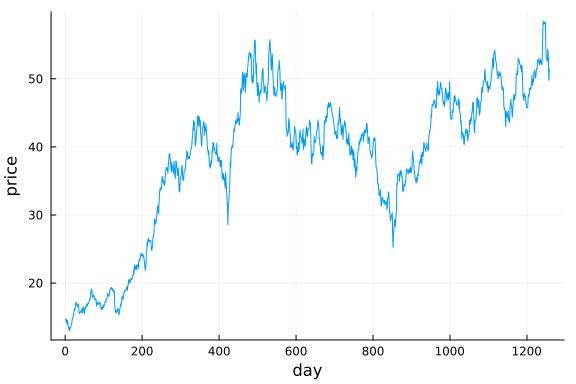
p_order = 10 # AR
q_order = 4 # MA4# Training set
train_size = 1000
x_prev_train = [Float64.(x_data[i+p_order-1:-1:i]) for i in 1:length(x_data)-p_order][1:train_size]
x_train = Float64.(x_data[p_order+1:end])[1:train_size];# Test set
x_prev_test = [Float64.(x_data[i+p_order-1:-1:i]) for i in 1:length(x_data)-p_order][train_size+1:end]
x_test = Float64.(x_data[p_order+1:end])[train_size+1:end];Inference
# Constraints are needed for performing VMP
arma_constraints = @constraints begin
    q(z, h_0, h, η, τ, γ,e) = q(h_0)q(z, h)q(η)q(τ)q(γ)q(e)
end;
# This cell defines prior knowledge for model parameters
h_prior = MvNormalMeanPrecision(zeros(q_order), diageye(q_order))
γ_prior = GammaShapeRate(1e4, 1.0)
τ_prior = GammaShapeRate(1e2, 1.0)
η_prior = MvNormalMeanPrecision(zeros(q_order), diageye(q_order))
θ_prior = MvNormalMeanPrecision(zeros(p_order), diageye(p_order));# Model's graph has structural loops, hence, it requires pre-initialisation
arma_initialization = @initialization begin
q(h_0) = h_prior
μ(h_0) = h_prior
q(h) = h_prior
μ(h) = h_prior
q(γ) = γ_prior
q(τ) = τ_prior
q(η) = η_prior
q(θ) = θ_prior
end
arma_meta = ar_meta(Multivariate, q_order, ARsafe());c = zeros(p_order); c[1] = 1.0; # AR
b = zeros(q_order); b[1] = 1.0; # MA
S = shift(q_order); # MA
result = infer(
model = ARMA(x_prev=x_prev_train, h_prior=h_prior, γ_prior=γ_prior, τ_prior=τ_prior, η_prior=η_prior, θ_prior=θ_prior, c=c, b=b, S=S),
data = (x = x_train, ),
initialization = arma_initialization,
constraints = arma_constraints,
meta = arma_meta,
iterations = 10,
options = (limit_stack_depth = 400, ),
);plot(mean.(result.posteriors[:e][end]), ribbon = var.(result.posteriors[:e][end]), label = "eₜ")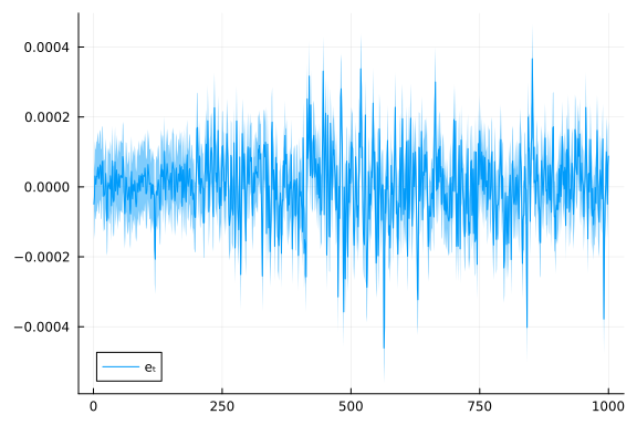
# extract posteriors
h_posterior = result.posteriors[:h][end][end]
γ_posterior = result.posteriors[:γ][end]
τ_posterior = result.posteriors[:τ][end]
η_posterior = result.posteriors[:η][end]
θ_posterior = result.posteriors[:θ][end];
Prediction
Here we are going to use our inference results in order to predict the dataset itself
# The prediction function is aimed at approximating the predictive posterior distribution
# It triggers the rules in the generative order (in future, RxInfer.jl will provide this function out of the box)
function prediction(x_prev, h_posterior, γ_posterior, τ_posterior, η_posterior, θ_posterior, p, q)
    h_out = MvNormalMeanPrecision(mean(h_posterior), precision(h_posterior))
    ar_out = @call_rule AR(:y, Marginalisation) (m_x=h_out, q_θ=η_posterior, q_γ=τ_posterior, meta=ARMeta(Multivariate, p, ARsafe()))
    c = zeros(p); c[1] = 1.0
    b = zeros(q); b[1] = 1.0
    ar_dot_out = @call_rule typeof(dot)(:out, Marginalisation) (m_in1=PointMass(b), m_in2=ar_out)
    θ_out = MvNormalMeanPrecision(mean(θ_posterior), precision(θ_posterior))
    ma_dot_out = @call_rule typeof(dot)(:out, Marginalisation) (m_in1=PointMass(x_prev), m_in2=θ_out)
    e_out = @call_rule NormalMeanPrecision(:out, Marginalisation) (q_μ=PointMass(0.0), q_τ=mean(γ_posterior))
    ar_ma = @call_rule typeof(+)(:out, Marginalisation) (m_in1=ar_dot_out, m_in2=ma_dot_out)
    @call_rule typeof(+)(:out, Marginalisation) (m_in1=ar_ma, m_in2=e_out)
end
prediction (generic function with 1 method)predictions = []
for x_prev in x_prev_test
push!(predictions, prediction(x_prev, h_posterior, γ_posterior, τ_posterior, η_posterior, θ_posterior, p_order, q_order))
# after every new prediction we can actually "retrain" the model to use the power of Bayesian approach
# we will skip this part at this notebook
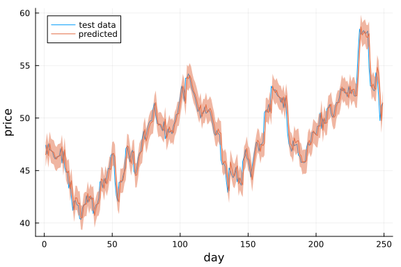
endplot(x_test, label="test data", legend=:topleft)
plot!(mean.(predictions)[1:end], ribbon=std.(predictions)[1:end], label="predicted", xlabel="day", ylabel="price")